Image Processing using CNN

convolutional-neural-net

Published

July 6, 2023

click here to read this in medium

Convolutional Neural Network

Basics →

What is an Image?

An image is nothing but an array of elements called pixels. A pixel is the smallest unit of a digital image or graphic that can be displayed and represented on a digital display device, which ranges between 0 and 255.
So, image is nothing but an n * 2d Array with values ranging from 0 to 255.
Note :- n depends on type of image, if the image is represented in RGB the n will be in 3.

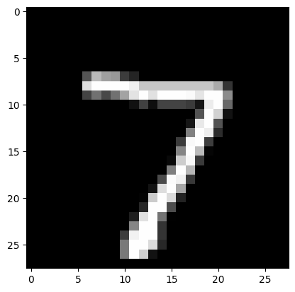
We are using MNIST dataset each image is a 28X28 pixel square. Which means we will be having 1 * 28 * 28 resolution images in our dataset. Let’s get the dataset and display the image😃.

import tensorflow as tf
import numpy as np
from matplotlib import pyplot as plt
from tensorflow.keras import utils as np_utils
(X_train,y_train),(X_test,y_test) = tf.keras.datasets.mnist.load_data()
X_test = X_test.reshape(X_test.shape[0], 1,28,28).astype('float32')
X_test = X_test/255
y_test = np_utils.to_categorical(y_test)
y_test = y_test/255
first_image = np.array(X_test[0], dtype='float')
pixels = first_image.reshape((28, 28))
plt.imshow(pixels, cmap='gray')
plt.show()

Introduction :-

CNN contains three type of layers which are

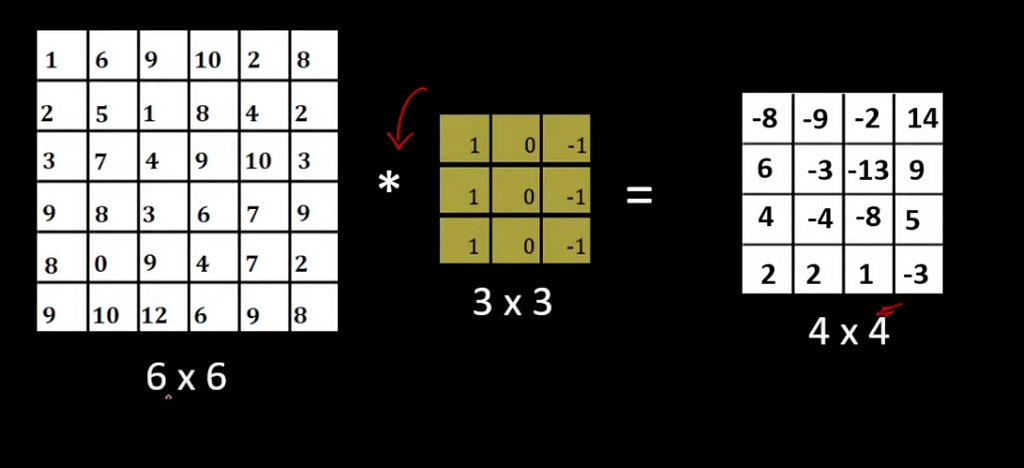
Convolutional Layer — Here we will be extracting the features present in the image. Example we can find all the horizontal lines present in the image using dot product of our horizontal matrix with the image matrix, then the resultant matrix will only contain the horizontal lines.

horizontal lines from the image source coding lane

Illustration of Convolution Operation(source)

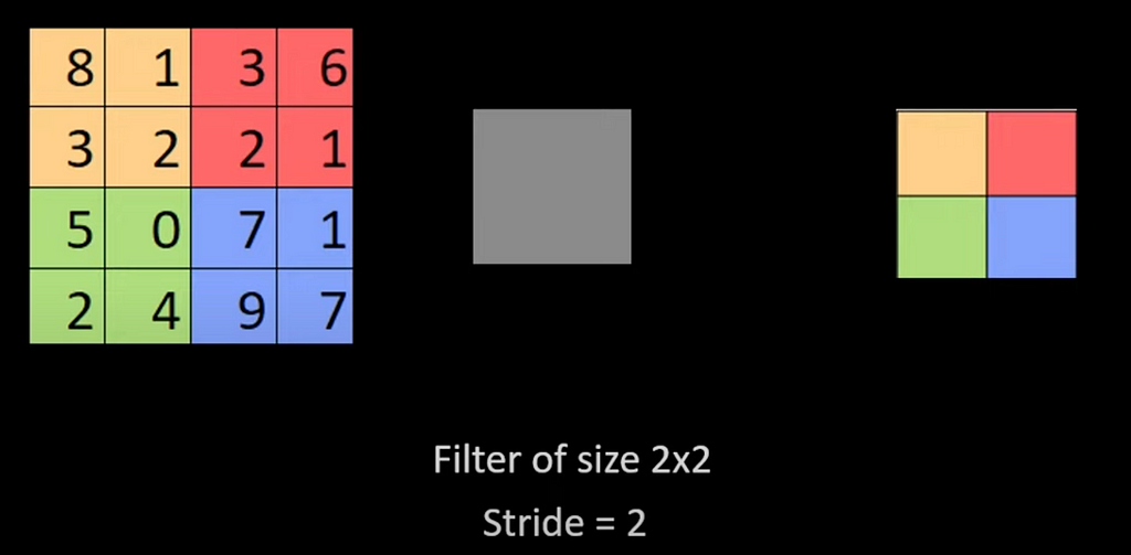
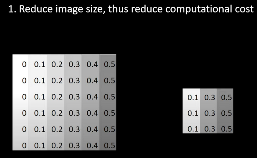
Pooling Layer — It is used to reduce the image size. By simply doing dot product for the image with a fixed slider.

Fully-Connected layer — Here it flattens the pixels and learns to associate features by forming all the combinations of flatten objects.

Let’s jump on the task

we have a dataset which contains digits from 0 to 9 in the form of images. Our task is to build a CNN model to predict the digit. So out CNN layers will be in this form.

Output Layer
(10 outputs)
Hidden Layer
(128 neurons)
Flatten Layer
Dropout Layer
20%
Max Pooling Layer
2×2
Convolutional Layer
32 maps, 5×5
Visible Layer
1x28x28

The first hidden layer is a Convolutional layer called Convolution2D. It consists of 32 feature maps with a size of 5×5 and uses the rectifier activation function.
The next layer is a pooling layer called MaxPooling2D. It performs 2×2 pooling, which means it takes the maximum value from a 2×2 grid of values.
A dropout layer follows, which helps with regularization. It randomly excludes 20% of the neurons in the layer during training to prevent overfitting.
The fifth layer is a flattened layer called Flatten. It converts the 2D matrix data from the previous layer into a 1D vector, allowing it to be processed by a fully connected layer.
Next, there is a fully connected layer with 128 neurons and the rectifier activation function.
Finally, the output layer consists of 10 neurons, representing the 10 classes in the classification task. It uses the softmax activation function to produce probability-like predictions for each class.

Coding it:

import numpy as np
from matplotlib import pyplot as plt
from tensorflow.keras.utils import to_categorical
from keras.models import Sequential
from keras.layers import Dense
from tensorflow.keras import utils as np_utils
from keras.layers import Dropout
from keras.layers import Flatten
from tensorflow.keras.layers import Conv2D
from tensorflow.keras.layers import MaxPooling2D
import tensorflow as tf
import time

#importing and preprocessing
(X_train,y_train), (X_test, y_test)= tf.keras.datasets.mnist.load_data()
X_train=X_train.reshape(X_train.shape[0], 1,28,28).astype('float32')
X_test=X_test.reshape(X_test.shape[0], 1,28,28).astype('float32')

X_train=X_train/255
X_test=X_test/255
y_train = np_utils.to_categorical(y_train)
y_test= np_utils.to_categorical(y_test)
num_classes=y_train.shape[1]
print(num_classes)

#prepare your model
def cnn_model():
    model=Sequential()
    # Convolutional Layer 32 map 5X5 and input 1 * 28 * 28
    model.add(Conv2D(32,5,5, padding='same',input_shape=(1,28,28), activation='relu'))
    # Max Pooling Layer 2 X 2
    model.add(MaxPooling2D(pool_size=(2,2), padding='same'))
    # Dropout Layer 20%
    model.add(Dropout(0.2))
    # Flatten Layer
    model.add(Flatten())
    # Hidden Layer 128 neurons
    model.add(Dense(128, activation='relu'))
    # Output Layer
    model.add(Dense(num_classes, activation='softmax'))
    model.compile(loss='categorical_crossentropy', optimizer='adam', metrics=['accuracy'])
    return model

t1 = time.time_ns()
model=cnn_model()
model.fit(X_train, y_train, validation_data=(X_test,y_test),epochs=10, batch_size=200, verbose=2)
t2 = time.time_ns()
score= model.evaluate(X_test, y_test, verbose=0)
t3 = time.time_ns()
train_time = t2-t1
evaluavation_time = t3-t2
print('The accuracy is: %.2f%%'%(score[1]))
print(f'training time {train_time}, evaluvation time {evaluavation_time}')

first_image = np.array(X_test[0], dtype='float')
pixels = first_image.reshape((28, 28))
plt.imshow(pixels, cmap='gray')
plt.show()
t4 = time.time_ns()
test_input = first_image.reshape((-1, 1, 28, 28))
k = model.predict(test_input).tolist()
t5 = time.time_ns()
print(f'predicted output : {k[0].index(max(k[0]))}')
print(f'actual output : {y_test[0]}')
print(f'prediction time {t5-t4}')

Results

Accuracy — 97%
Training run time — 7.2892 Sec
Evaluation run time — 0.186776 Sec
Prediction run time (for digit 7) — 0.033601 Sec

Complete code is available in my GitHub (https://github.com/propardhu/Pandas_Play/blob/main/CNN_mnist.ipynb)

https://medium.com/media/9602ed028d76e3f631dae05408c7e2cd/href